geoExposeR: Environmental Exposure Health Modeling • geoExposeR

An R package for modeling health effects of environmental exposures, with a primary focus on groundwater contaminants, based on epidemiological studies and existing concentration models.

USGS IPDS Record Number: IP-180903

Citation

If you use geoExposeR in your research, please cite the software release:

Majumdar, S., Bartell, S. M., Lombard, M. A., Smith, R. G., and Gribble, M. O., 2026, geoExposeR: An R package for modeling health effects of environmental exposures: U.S. Geological Survey software release, https://doi.org/10.5066/P1JGUKMD

BibTeX:

@software{majumdar2026geoExposeR,
  title={geoExposeR: An R package for modeling health effects of environmental exposures},
  author={Majumdar, Sayantan and Bartell, Scott M and Lombard, Melissa A and Smith, Ryan G and Gribble, Matthew O},
  year={2026},
  publisher={U.S. Geological Survey},
  note={U.S. Geological Survey Software Release},
  doi={10.5066/P1JGUKMD},
  url={https://doi.org/10.5066/P1JGUKMD}
}

And the accompanying paper (under review at JOSS):

Majumdar, S., Bartell, S. M., Lombard, M. A., Smith, R. G., and Gribble, M. O., 2026, geoExposeR: An R package for modeling health effects of environmental exposures, Journal of Open Source Software (under review).

BibTeX:

@article{majumdar2026geoExposeRpaper,
  title={geoExposeR: An R package for modeling health effects of environmental exposures},
  author={Majumdar, Sayantan and Bartell, Scott M and Lombard, Melissa A and Smith, Ryan G and Gribble, Matthew O},
  journal={Journal of Open Source Software},
  year={2026},
  note={Under review},
  url={https://code.usgs.gov/envirohealth/geoExposeR}
}

Statement of Need
Workflow
Installation
Quick Start
Examples
Package Structure
Core Functions
Key Features
Documentation
Data Requirements
Data Preparation Workflow
Running Tests
Modifying the R Package
Contributing
Troubleshooting
License

Statement of Need

Environmental epidemiologists face a fundamental challenge: exposure to environmental contaminants is rarely measured directly for study participants. Instead, researchers must estimate exposures using predictive models, monitoring data, or biomarkers—each with inherent uncertainty. Failing to account for this uncertainty can lead to biased effect estimates and misleading conclusions about health risks (Majumdar and others, 2026).

This challenge is particularly acute for drinking water contaminants like arsenic, where an estimated 40 million Americans rely on unregulated private wells. Foundational studies developed sophisticated methods to address exposure uncertainty by combining U.S. Geological Survey (USGS) machine learning predictions with U.S. Environmental Protection Agency (EPA) monitoring data through population-weighted integration and multiple imputation. However, implementing these methods requires specialized expertise in geospatial analysis, statistical modeling, and R programming—presenting a significant barrier for many researchers.

geoExposeR directly addresses this need by packaging the complete analytical pipeline into accessible R functions. The package automates:

Integration of probabilistic exposure estimates from multiple data sources
Population-weighted combination of exposure probabilities
Multiple imputation to propagate exposure uncertainty
Configurable regression modeling—fixed-, random-, or mixed-effects structures in linear, generalized, or multinomial form—with proper clustering adjustment
Result pooling via Rubin’s Rules with appropriate variance estimation

While designed for drinking water arsenic exposure assessments, the underlying statistical framework is broadly applicable to other environmental contaminants (nitrate, uranium, manganese, PFAS) and air pollutants (PM2.5, ozone) where probabilistic exposure estimates and health outcome data are available. The package includes worked examples for nitrate (infant methemoglobinemia), uranium (kidney function), and PM2.5 (respiratory outcomes), demonstrating how the framework generalizes to other contaminants and health endpoints. See the Broader Applicability section and example scripts for guidance on adapting the package to other domains.

By lowering technical barriers to rigorous uncertainty quantification, geoExposeR promotes reproducibility and enables wider application of state-of-the-art methods in environmental epidemiology.

For a detailed description of the methodology, see Majumdar and others (2026).

Terminology: Two Input Data Types

The package combines two distinct types of input data using population-based weights (e.g., private well vs. public water usage) to create integrated exposure probability distributions:

Parameter Data Type Description Examples

model_prob_csv Modeled probabilistic estimates Multinomial probability distributions across concentration categories, typically derived from predictive models USGS machine learning predictions, satellite-derived estimates, hybrid spatial models

conc_data_csv Measured concentrations Point measurements or summary statistics of contaminant concentrations from monitoring stations or laboratory analyses EPA public water system monitoring, ground-based air quality monitors, field sampling data

Any dataset that provides modeled probabilities can serve as the probability input (model_prob_csv), and any dataset that provides measured concentrations can serve as the concentration input (conc_data_csv), regardless of the originating agency.

Parameter	Data Type	Description	Examples
`model_prob_csv`	Modeled probabilistic estimates	Multinomial probability distributions across concentration categories, typically derived from predictive models	USGS machine learning predictions, satellite-derived estimates, hybrid spatial models
`conc_data_csv`	Measured concentrations	Point measurements or summary statistics of contaminant concentrations from monitoring stations or laboratory analyses	EPA public water system monitoring, ground-based air quality monitors, field sampling data

Workflow

The figure below illustrates the complete analytical workflow implemented in geoExposeR. The pipeline integrates four input data sources through data ingestion, probability integration, multiple imputation, and statistical modeling stages to produce pooled estimates with proper uncertainty quantification.

geoExposeR Workflow

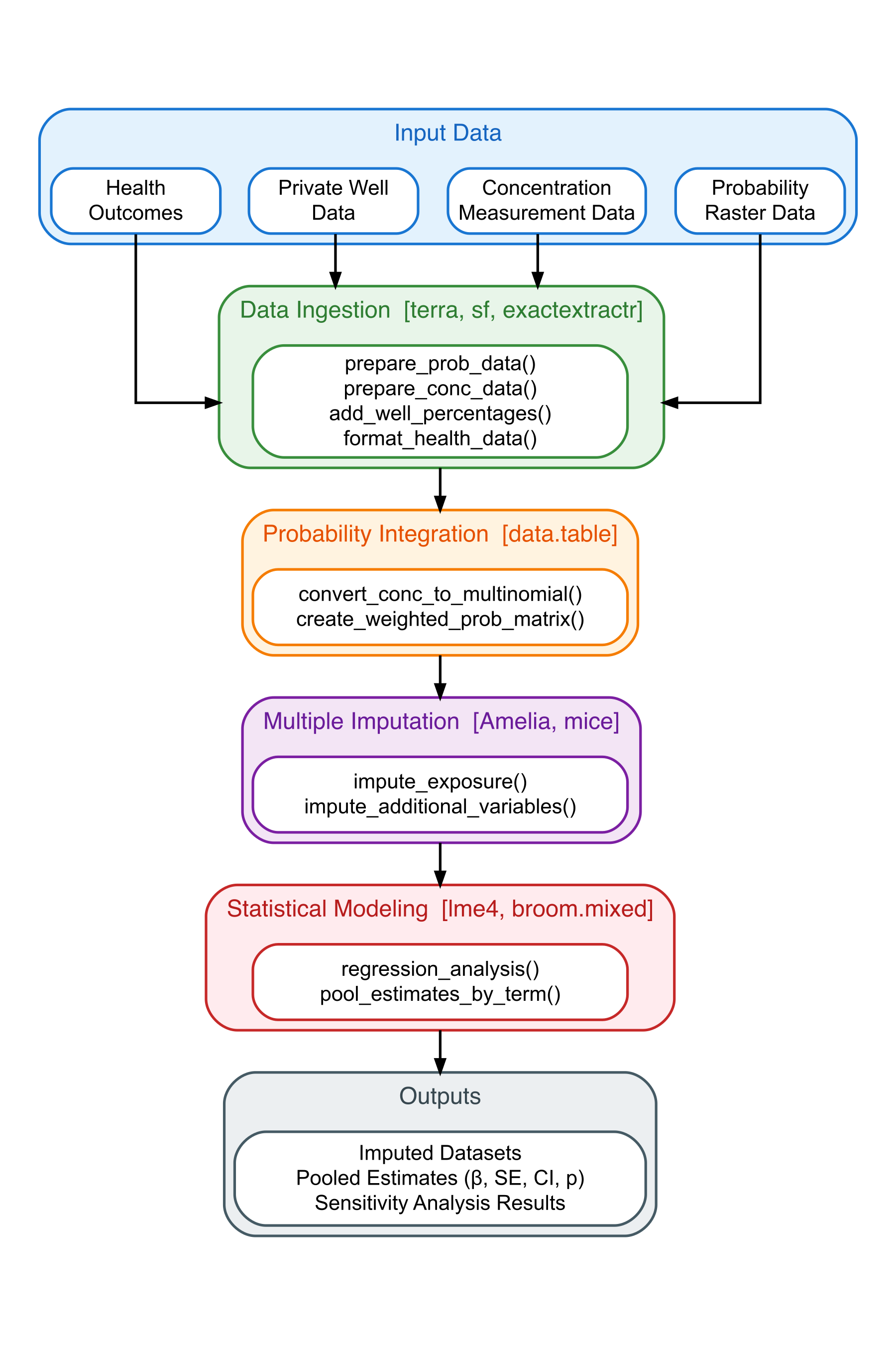
geoExposeR analytical workflow showing the data processing pipeline from input sources through statistical modeling to pooled estimates. Packages used at each stage are indicated in brackets. Pooled estimates include regression coefficients (β), standard errors (SE), 95% confidence intervals (CI), and p-values, all computed using Rubin’s Rules. Adapted from Majumdar and others (2026).

Key Capabilities

Category	Features
Data Ingestion	Process GeoTIFF rasters, concentration measurements, health data; geographic subsetting; input validation
Exposure Modeling	Probability/concentration data integration; population-weighted averaging; lognormal parameter estimation
Statistical Analysis	Multiple imputation (MICE); fixed-/random-/mixed-effects regression (linear, generalized, or multinomial); Rubin’s Rules pooling
Quality Assurance	100% test coverage; comprehensive input validation; reproducible workflows

Existing methods from studies like Bulka and others (2022) and Lombard and others (2021) provide robust statistical frameworks but require complex implementation involving: - Integration of multiple probabilistic models (modeled probabilities and measured concentrations) - Multiple imputation techniques for uncertain exposures - Mixed-effects regression with proper pooling of results

geoExposeR solves this by packaging these sophisticated methods into user-friendly functions. This enables researchers to:

🔬 Focus on science, not statistical programming
📊 Ensure reproducibility across studies
⚡ Accelerate research on environmental health effects
🎯 Apply best practices for uncertainty quantification
🗺️ Work with multiple data formats (GeoTIFF, CSV, shapefiles)

By democratizing access to these methods, geoExposeR promotes more rigorous and comparable environmental exposure research.

Installation

System Dependencies: Pandoc

To build the package vignettes, which provide detailed documentation and examples, you need to have Pandoc installed. RStudio bundles a version of Pandoc, so if you are an RStudio user, you may not need to install it separately.

If you do not have Pandoc, you can download and install it from the official website: pandoc.org/installing.html.

R Package Installation

Prerequisites: R (≥ 4.4.0) and Pandoc for building vignettes.

Install from USGS GitLab:

Note: These commands will work once the repository is approved and publicly available, with the tag/branch suffix pointing to a tagged release version. The devtools::install_*() helpers were deprecated in devtools 2.5.0 in favor of pak, so the examples below use pak.

# Install pak if not already installed
if (!require("pak")) install.packages("pak")

# Install geoExposeR from USGS GitLab (specific tag or branch)
pak::pak("git::https://code.usgs.gov/envirohealth/geoExposeR.git@v1.0.0")  # Replace with desired tag or branch (e.g. @main)

# Load the package
library(geoExposeR)

pak does not build vignettes by default. To build the vignettes locally during installation, use the non-deprecated remotes::install_git(), which also supports the self-hosted code.usgs.gov host:

# install.packages("remotes")
remotes::install_git(
  "https://code.usgs.gov/envirohealth/geoExposeR.git",
  ref = "v1.0.0",  # Replace with desired tag or branch (e.g. "main")
  build_vignettes = TRUE
)

For development and testing (includes coverage tools):

# Install additional development dependencies
install.packages(c("pak", "testthat", "covr", "DT", "htmltools"))

# Install geoExposeR from USGS GitLab (specific tag or branch)
pak::pak("git::https://code.usgs.gov/envirohealth/geoExposeR.git@main")  # Or use a specific tag like @v1.0.0

Verify installation:

# Check package version
packageVersion("geoExposeR")

# View help
?perform_sensitivity_analysis

Package Documentation Website:

The complete package documentation, including detailed function references, vignettes, and examples, is available at: https://envirohealth.code-pages.usgs.gov/geoExposeR/

This website is automatically generated and updated whenever changes are made to the main branch, ensuring you always have access to the latest documentation.

Local Installation from Downloaded ZIP

If you downloaded the repository as a ZIP file (e.g., from GitLab or GitHub), you can install the package locally:

Extract the ZIP file to a directory of your choice.
Install from the extracted folder:

# Install devtools if not already installed
if (!require("devtools")) install.packages("devtools")

# Install from the local directory
# Replace the path with the actual path to the extracted folder
devtools::install_local(
  path = "/path/to/geoExposeR",  # Path to the extracted package folder
  build_vignettes = TRUE,
  dependencies = TRUE
)

# Load the package
library(geoExposeR)

Alternative: Install from the ZIP file directly (without extracting):

# Install directly from the ZIP file
devtools::install_local(
  path = "/path/to/geoExposeR.zip",  # Path to the downloaded ZIP file
  build_vignettes = TRUE,
  dependencies = TRUE
)

Using RStudio:

You can also install the package using RStudio’s GUI: 1. Go to Tools > Install Packages… 2. In the “Install from:” dropdown, select Package Archive File (.zip; .tar.gz) 3. Click Browse and navigate to the downloaded ZIP or tarball file 4. Click Install

Note: Building vignettes requires Pandoc. If you encounter issues, you can skip vignette building by setting build_vignettes = FALSE.

Modifying the R Package

If you want to customize this package, run the following using R after you have modified the codes.

# Set the working directory to your package directory
setwd(<path to geoExposeR>)

# Load devtools
library(devtools)

# Generate documentation
document()

# Build the package
build()

# Install the package
install()

Quick Start

library(geoExposeR)

# Run sensitivity analysis with your data
results <- perform_sensitivity_analysis(
  ndraws = 10,
  model_prob_csv = "path/to/prob_data.csv",
  conc_data_csv = "path/to/conc_data.csv",
  birth_data_txt = "path/to/birth_data.txt",
  regression_formula = "~ ExposureLevel + MAGE_R + rural + (1|FIPS)",
  output_dir = "results/",
  targets = c("OEGEST", "BWT")
)

# View results
print(results)

Using Raw Concentration Data

If your concentration data contains raw values instead of pre-calculated lognormal parameters, specify the concentration column and the package will automatically convert them:

results <- perform_sensitivity_analysis(
  ndraws = 10,
  model_prob_csv = "path/to/prob_data.csv",
  conc_data_csv = "path/to/conc_raw.csv",     # File with raw concentrations
  conc_raw_col = "concentration",            # Column with raw values
  default_sdlog = 1.0,                      # Default sdlog value
  birth_data_txt = "path/to/birth_data.txt",
  regression_formula = "~ ExposureLevel + MAGE_R + rural + (1|FIPS)",
  output_dir = "results/",
  targets = c("OEGEST", "BWT")
)

For detailed examples with dummy data, see the vignette.

Examples

The package includes multiple working examples in the examples/ folder that demonstrate different workflows for using geoExposeR.

Available Examples

Core Arsenic Examples

Example File	Description
`run_geoExposeR_example.R`	Basic example using pre-formatted CSV data
`run_geoExposeR_from_geotiff.R`	Complete GeoTIFF workflow from rasters to analysis
`run_geoExposeR_data_pipeline.R`	Demonstrates all data ingestion functions
`run_geoExposeR_model_variants.R`	Fixed-, random-, and mixed-effects models in linear, non-linear (logistic/Poisson), and multinomial variants
`run_geoExposeR_fixed_multi_target.R`	Fixed-effects models over multiple targets at once, including binary categorical (character and 0/1) outcomes via logistic regression and multi-level categorical outcomes via multinomial regression

Broader Application Examples

These examples demonstrate how geoExposeR can be adapted for other environmental contaminants and exposures:

Example File	Contaminant	Health Outcome	Description
`run_geoExposeR_nitrate.R`	Nitrate	Methemoglobinemia	Groundwater nitrate effects on infant health
`run_geoExposeR_uranium.R`	Uranium	Kidney function (eGFR)	Groundwater uranium nephrotoxicity
`run_geoExposeR_pm25.R`	PM2.5	Respiratory function (FEV1)	Air quality effects on lung function

Running the Examples

# From the geoExposeR directory
cd /path/to/geoExposeR

# Basic example (CSV workflow)
Rscript examples/run_geoExposeR_example.R

# GeoTIFF workflow example
Rscript examples/run_geoExposeR_from_geotiff.R

# Data pipeline example (all ingestion functions)
Rscript examples/run_geoExposeR_data_pipeline.R

# Model variants (fixed/random/mixed, linear and non-linear)
Rscript examples/run_geoExposeR_model_variants.R

# Fixed-effects models over multiple targets, including categorical outcomes
Rscript examples/run_geoExposeR_fixed_multi_target.R

# Broader application examples
Rscript examples/run_geoExposeR_nitrate.R
Rscript examples/run_geoExposeR_uranium.R
Rscript examples/run_geoExposeR_pm25.R

Or in R/RStudio:

# Set working directory to package root
setwd("/path/to/geoExposeR")

# Run basic example
source("examples/run_geoExposeR_example.R")

# Run GeoTIFF workflow
source("examples/run_geoExposeR_from_geotiff.R")

# Run data pipeline demo
source("examples/run_geoExposeR_data_pipeline.R")

# Run broader application examples
source("examples/run_geoExposeR_nitrate.R")
source("examples/run_geoExposeR_uranium.R")
source("examples/run_geoExposeR_pm25.R")

Example Data Files

The examples use data files from the examples/input_data/ folder:

Core Arsenic Data

File	Description
`prob_dom.csv`	Modeled multinomial probabilities of arsenic levels (50 rows)
`conc_dom.csv`	Measured arsenic concentration data (50 rows)
`Demographics_dom.txt`	Demographics data with health outcomes - SBP (50 rows)

Broader Application Data

File	Description
`prob_nitrate.csv`	Modeled nitrate probability data for infant health example (50 rows)
`conc_nitrate.csv`	Measured nitrate concentration data (50 rows)
`Health_nitrate.txt`	Infant methemoglobin and birth weight data (50 rows)
`prob_uranium.csv`	Modeled uranium probability data for kidney function example (50 rows)
`conc_uranium.csv`	Measured uranium concentration data (50 rows)
`Health_uranium.txt`	Kidney function (eGFR) and demographic data (50 rows)
`prob_pm25.csv`	Modeled PM2.5 probability estimates (50 rows)
`conc_pm25.csv`	Measured PM2.5 concentration data (50 rows)
`Health_pm25.txt`	Respiratory function (FEV1) and smoking data (50 rows)

⚠️ Note on Example Data: All example data files are simulated dummy data created for demonstration and testing purposes only. The county-level exposure files contain 50 synthetic counties, and the health file contains ~400 synthetic individual-level records nested within those counties (multiple participants per county, which makes a geographic random intercept (1 | id) identifiable). They have realistic column structures but randomly generated values. The actual research data cannot be shared publicly due to data use agreements and privacy restrictions. The dummy data preserves the structure and format of the real data to allow users to understand the workflow and test the package functionality.

Example 1: Basic CSV Workflow (`run_geoExposeR_example.R`)

Demonstrates the standard analysis workflow using pre-formatted CSV data:

Data Loading: Using custom column names to work with original data formats
Concentration Data Preprocessing: Converting raw concentrations to lognormal parameters
Custom Column Mapping: Specifying non-standard column names via function parameters
Sensitivity Analysis: Running multiple imputation with mixed-effects regression
Result Interpretation: Understanding the pooled estimates and confidence intervals

Example 2: GeoTIFF Workflow (`run_geoExposeR_from_geotiff.R`)

Demonstrates processing raw GeoTIFF raster data through the complete analysis pipeline:

Creating GeoTIFF Rasters: Generating mock probability surfaces (P(As > 5), P(As > 10))
Creating Boundaries: Building geographic polygons for extraction
Extracting Probabilities: Using prepare_prob_data() to extract probabilities by geographic unit
Processing Concentration Data: Using prepare_conc_data() to compute lognormal parameters
Formatting Health Data: Using format_health_data() to standardize outcomes
Validating Inputs: Using validate_prepared_inputs() for quality control
Running Analysis: Executing the full sensitivity analysis

Example 3: Data Pipeline Demo (`run_geoExposeR_data_pipeline.R`)

Comprehensively demonstrates all data ingestion functions:

prepare_conc_data(): Raw vs. summary concentration input types, population weighting
format_health_data(): Identifier formatting, multiple outcome support
add_well_percentages(): Merging private well population data
subset_by_geography(): Filtering by state FIPS codes or GEOID lists
validate_prepared_inputs(): Input file validation

Key Features Shown

Using id_col, prob_cols, pop_well_col for probability data mapping
Using conc_mean_col, conc_sd_col, pwell_col for concentration data mapping
Using record_id_col, exposure_level_col for health data mapping
Setting appropriate conc_cutoffs for concentration categorization
Configuring MICE imputation parameters (mice_m, mice_maxit, mice_method)
Processing GeoTIFF rasters with terra and sf packages
Geographic subsetting by state or custom GEOID lists

Package Structure

The geoExposeR package follows the standard structure for R packages:

geoExposeR/
├── R/                                  # Source code
│   ├── geoExposeR.R                    # Main exported function
│   ├── data-loading.R                  # Data loading and processing
│   ├── data-ingestion.R                # Raw data preparation (GeoTIFF, concentration, health)
│   ├── imputation.R                    # Multiple imputation functions
│   ├── regression.R                    # Regression analysis and pooling
│   └── utils.R                         # Validation and utility functions
├── man/                                # Generated documentation (.Rd files)
├── examples/
│   ├── run_geoExposeR_example.R        # Basic CSV workflow example
│   ├── run_geoExposeR_from_geotiff.R   # GeoTIFF raster workflow
│   ├── run_geoExposeR_data_pipeline.R  # Data ingestion functions demo
│   ├── run_geoExposeR_model_variants.R # Fixed/random/mixed model variants
│   ├── run_geoExposeR_fixed_multi_target.R # Fixed-effects, multiple targets
│   ├── run_geoExposeR_nitrate.R        # Nitrate exposure example
│   ├── run_geoExposeR_uranium.R        # Uranium exposure example
│   ├── run_geoExposeR_pm25.R           # PM2.5 air quality example
│   ├── input_data/                     # Example input data files (all dummy data*)
│   │   ├── generate_demographics.R     # Reproducible generator for Demographics_dom.txt
│   │   ├── prob_dom.csv                # Sample arsenic probability data (dummy*)
│   │   ├── conc_dom.csv                # Sample arsenic concentration data (dummy*)
│   │   ├── Demographics_dom.txt        # Sample individual-level health data (dummy*)
│   │   ├── prob_nitrate.csv            # Sample nitrate probability data (dummy*)
│   │   ├── conc_nitrate.csv            # Sample nitrate concentration data (dummy*)
│   │   ├── Health_nitrate.txt          # Sample infant health data (dummy*)
│   │   ├── prob_uranium.csv            # Sample uranium probability data (dummy*)
│   │   ├── conc_uranium.csv            # Sample uranium concentration data (dummy*)
│   │   ├── Health_uranium.txt          # Sample kidney function data (dummy*)
│   │   ├── prob_pm25.csv              # Sample PM2.5 probability data (dummy*)
│   │   ├── conc_pm25.csv              # Sample PM2.5 concentration data (dummy*)
│   │   └── Health_pm25.txt             # Sample respiratory health data (dummy*)
├── tests/
│   ├── testthat/
│   │   └── test-geoExposeR.R           # Comprehensive test suite (557 tests)
│   └── testthat.R                      # Test runner
├── vignettes/
│   └── geoExposeR-vignette.Rmd         # Package tutorial and examples
├── paper/                              # JOSS paper files
│   ├── paper.md                        # Paper manuscript
│   ├── paper.bib                       # References
│   ├── generate_workflow_figure.R      # Script to generate workflow diagram
│   ├── workflow.png                    # Workflow diagram (600 DPI)
├── docs/                               # pkgdown generated website
├── .gitlab-ci.yml                      # GitLab CI/CD pipeline configuration
├── .gitignore                          # Git ignore patterns
├── .Rbuildignore                       # R build ignore patterns
├── _pkgdown.yml                        # pkgdown website configuration
├── code.json                           # USGS code.json metadata
├── CONTRIBUTING.md                     # Contribution guidelines
├── DESCRIPTION                         # Package metadata and dependencies
├── DISCLAIMER.md                       # USGS disclaimer
├── LICENSE.md                          # CC0 1.0 Universal license
├── NAMESPACE                           # Package exports and imports
├── NEWS.md                             # Change log and version history
└── README.md                           # This file

*Dummy data for demonstration; actual research data cannot be shared.

R/ Directory Structure

The package uses a modular architecture with functionality organized across specialized files:

geoExposeR.R: Main exported function perform_sensitivity_analysis()
data-loading.R: Data loading and probability matrix processing
data-ingestion.R: Functions to prepare data from raw sources (GeoTIFFs, concentration measurements, health data)
imputation.R: Multiple imputation using MICE framework
regression.R: Mixed-effects regression and Rubin’s Rules pooling
utils.R: Input validation and utility functions

This approach provides several advantages: - Separation of concerns: Each file handles a specific domain - Easier testing: Functions can be tested in isolation - Better maintainability: Changes are localized to specific modules - Clearer organization: Easy to find relevant code

Testing Infrastructure

The package includes comprehensive testing with 100% code coverage:

tests/testthat/test-geoExposeR.R: Main test suite with 557 tests (includes helper functions)
tests/testthat.R: Standard R package test runner
.gitlab-ci.yml: GitLab CI/CD pipeline with automated testing and coverage reporting

Key Internal Functions

While users primarily interact with perform_sensitivity_analysis(), the package includes several internal functions organized by functionality:

Data Loading (data-loading.R): - load_and_process_exposure_data(): Orchestrates modeled probability and measured concentration data loading - load_prob_data(): Loads modeled probability data - convert_conc_to_multinomial(): Converts concentration lognormal parameters to multinomial probabilities - create_weighted_prob_matrix(): Creates weighted combined probability matrix - load_and_process_birth_data(): Loads and processes birth/health outcome data

Multiple Imputation (imputation.R): - impute_exposure(): Creates multiple imputed datasets with exposure levels - impute_additional_variables(): Imputes missing covariates using MICE - validate_imputed_datasets(): Validates imputation results

Regression Analysis (regression.R): - regression_analysis(): Fits the selected regression model (fixed/random/mixed effects; linear, generalized, or multinomial) on imputed data - pool_estimates_by_term(): Pools regression estimates using Rubin’s Rules - pool_single_estimate(): Applies Rubin’s Rules to individual parameters

Data Ingestion (data-ingestion.R): - prepare_prob_data(): Convert probability GeoTIFF rasters to CSV format - prepare_conc_data(): Process concentration data to lognormal parameters - format_health_data(): Format and validate health outcome data - add_well_percentages(): Merge private well population percentages - subset_by_geography(): Filter data by state, region, or custom area - validate_prepared_inputs(): Comprehensive validation of prepared files

Utilities (utils.R): - validate_all_inputs(): Input validation and error checking - format_ids_func(): Smart identifier formatting with automatic type detection (zero-pads numeric FIPS codes, preserves alphanumeric IDs) - Additional helper functions for data validation and formatting

Core Functions

Main Analysis Function

perform_sensitivity_analysis(): This is the main exported function of the package. It orchestrates the entire workflow from data loading through final analysis:

Data Loading: Loads and processes modeled probability data, measured concentration parameters, and birth/health outcome data
Probability Integration: Combines probability and concentration models using weighted averages based on private well usage
Multiple Imputation: Creates multiple datasets with probabilistically assigned exposure levels
Covariate Imputation: Optionally imputes missing values in additional covariates using MICE
Statistical Analysis: Fits regression models to assess exposure-outcome relationships, with selectable fixed-, random-, or mixed-effects structures in linear or non-linear (generalized) variants (see Regression Model Options)
Results Pooling: Applies Rubin’s Rules to pool results across imputed datasets
Output Generation: Saves results and returns structured analysis output

The function is designed to handle the complex statistical methodology while providing a simple, user-friendly interface that requires minimal statistical programming expertise.

Regression Model Options

perform_sensitivity_analysis() supports flexible regression model structures through two arguments, model_type and model_family. This lets you fit fixed-effects, random-effects, or mixed-effects models, each in a linear (Gaussian) or non-linear (generalized) variant.

model_type selects the effects structure:

`model_type`	Effects structure	Random terms in formula
`"fixed"`	Fixed effects only (no random effects)	Not allowed
`"random"`	Random intercepts only	Required, intercept-only, e.g. `(1 \\| county)`
`"mixed"` (default)	Fixed effects + random effects	Required, slopes allowed, e.g. `(1 \\| county)` or `(age \\| county)`

model_family selects the response distribution:

NULL (default): a linear model (Gaussian / identity link), for continuous outcomes.
A family name ("binomial", "poisson", …), a family object (e.g. poisson()), or a family-generating function: a non-linear generalized model, for binary, count, or other outcomes.
"multinomial": a multinomial logistic model for multi-level categorical outcomes (3+ categories). Fixed-effects fits use nnet::multinom(); random- and mixed-effects fits use mclogit::mblogit().

The combination selects the fitting engine automatically:

`model_type`	linear (`model_family = NULL`)	non-linear (`model_family` set)	multinomial (`model_family = "multinomial"`)
`"fixed"`	`stats::lm()`	`stats::glm()`	`nnet::multinom()`
`"random"`	`lme4::lmer()`	`lme4::glmer()`	`mclogit::mblogit()`
`"mixed"`	`lme4::lmer()`	`lme4::glmer()`	`mclogit::mblogit()`

Regardless of engine, coefficients are extracted for the exposure terms and pooled across imputed datasets using Rubin’s Rules. For non-linear models the pooled estimate q.mi is on the link scale (e.g. a log-odds ratio for "binomial"; exp(q.mi) gives the odds ratio). Multinomial results include an extra y.level column identifying the outcome category (relative to the reference level) that each pooled estimate refers to.

# Linear fixed-effects model (ordinary least squares)
perform_sensitivity_analysis(
  ...,
  regression_formula = "~ as.factor(ExposureLevel) + maternal_age",
  model_type = "fixed"            # model_family = NULL -> stats::lm()
)

# Linear random-intercept model
perform_sensitivity_analysis(
  ...,
  regression_formula = "~ as.factor(ExposureLevel) + (1 | county)",
  model_type = "random"          # -> lme4::lmer()
)

# Linear mixed-effects model (default)
perform_sensitivity_analysis(
  ...,
  regression_formula = "~ as.factor(ExposureLevel) + maternal_age + (1 | county)",
  model_type = "mixed"           # -> lme4::lmer()
)

# Non-linear (logistic) mixed-effects model for a binary outcome
perform_sensitivity_analysis(
  ...,
  targets = "preterm",
  regression_formula = "~ as.factor(ExposureLevel) + maternal_age + (1 | county)",
  model_type = "mixed",
  model_family = "binomial"      # -> lme4::glmer()
)

# Non-linear (Poisson) fixed-effects model for a count outcome
perform_sensitivity_analysis(
  ...,
  targets = "n_events",
  regression_formula = "~ as.factor(ExposureLevel) + maternal_age",
  model_type = "fixed",
  model_family = poisson()       # -> stats::glm()
)

See examples/run_geoExposeR_model_variants.R for a runnable demonstration of these combinations, including the multinomial fixed-, random-, and mixed-effects variants.

Categorical outcomes and multiple targets

A single perform_sensitivity_analysis() call applies one model_family to every target it is given, so outcomes of different types are best grouped into separate calls:

Continuous outcomes use a linear model (model_family = NULL).
Binary categorical outcomes use a logistic model (model_family = "binomial"). They may be supplied as a 0/1 indicator or as a two-level categorical column — a character outcome such as "high"/"normal" (as read from a text file) is automatically coerced to a factor before fitting, with the first level treated as the reference.
Multi-level categorical outcomes (3+ categories) use a multinomial model (model_family = "multinomial"). Character columns are coerced to factors automatically, and the pooled results gain a y.level column for the outcome category.

# Continuous outcomes -> linear fixed effects
continuous <- perform_sensitivity_analysis(
  ..., targets = c("BWT", "gestational_age"),
  model_type = "fixed", model_family = NULL
)

# Binary categorical outcomes -> logistic fixed effects
binary <- perform_sensitivity_analysis(
  ..., targets = c("preterm", "bp_category"),   # 0/1 or "high"/"normal"
  model_type = "fixed", model_family = "binomial"
)

# Multi-level categorical outcome -> multinomial fixed effects
multilevel <- perform_sensitivity_analysis(
  ..., targets = "bp_stage",   # e.g. "normal"/"elevated"/"stage2"
  model_type = "fixed", model_family = "multinomial"
)

results <- c(continuous, binary, multilevel)

See examples/run_geoExposeR_fixed_multi_target.R for a complete fixed-effects example spanning continuous, binary, and multi-level categorical outcomes.

Data Ingestion Functions

The package provides functions to help prepare input data from raw sources:

prepare_prob_data(): Extracts probabilities from GeoTIFF rasters and aggregates by geographic unit.

library(terra)
library(sf)

prob_data <- prepare_prob_data(
  prob_rasters = list(
    gt5 = "path/to/prob_gt5.tif",
    gt10 = "path/to/prob_gt10.tif"
  ),
  boundaries = county_boundaries,
  id_col = "GEOID",
  extraction_method = "mean",
  cutoffs = c(5, 10),
  output_file = "prob_data_output.csv"
)

prepare_conc_data(): Processes concentration measurements and converts to lognormal parameters.

conc_data <- prepare_conc_data(
  conc_data = raw_measurements,
  id_col = "county_fips",
  concentration_col = "arsenic_ug_L",
  population_col = "pop_served",
  input_type = "raw",
  output_file = "conc_lognormal.csv"
)

format_health_data(): Formats and validates health outcome data.

health_data <- format_health_data(
  health_data = raw_health_data,
  id_col = "FIPS",
  outcome_cols = c("BWT", "OEGEST"),
  covariate_cols = c("MAGE", "rural"),
  output_file = "health_outcomes.txt"
)

subset_by_geography(): Filters data to specific states or regions.

# Subset to California
ca_data <- subset_by_geography(
  data = prob_data,
  state_fips = "06"
)

# Subset to specific counties
selected <- subset_by_geography(
  data = prob_data,
  geoid_list = c("06001", "06003", "06005")
)

validate_prepared_inputs(): Validates all prepared input files before analysis.

validation <- validate_prepared_inputs(
  prob_file = "prob_data_output.csv",
  conc_file = "conc_lognormal.csv",
  health_file = "health_outcomes.txt"
)

if (validation$valid) {
  message("All files ready for analysis!")
}

Broader Applicability

While geoExposeR was designed for arsenic exposure assessment, the underlying statistical framework is fully adaptable to other environmental contaminants and exposures. The package’s methodology—combining probabilistic exposure estimates with health outcome data through multiple imputation—applies to any exposure assessment problem with similar data structures.

Supported Applications

Domain	Contaminants	Example Health Outcomes
Groundwater	Arsenic, Nitrate, Uranium, Manganese, PFAS	Birth outcomes, kidney function, neurological effects
Air Quality	PM2.5, Ozone, Wildfire smoke, NO₂	Respiratory function, cardiovascular disease, mortality
Soil/Dust	Lead, Heavy metals	Blood lead levels, cognitive development

Adapting geoExposeR for Other Contaminants

The package parameters map naturally to any two probability/concentration data sources:

Package Parameter	Arsenic Example	Nitrate Example	PM2.5 Example
`model_prob_csv`	Machine learning predictions	Nitrate model predictions	Satellite/hybrid estimates
`conc_data_csv`	Public water monitoring data	PWS nitrate measurements	Ground monitor data
`conc_cutoffs`	`c(5, 10)` µg/L	`c(5, 10)` mg/L NO₃-N	`c(9, 35)` µg/m³
Health outcome	Birth weight, SBP	Methemoglobin levels	FEV1 % predicted

Example: Adapting for Nitrate

# Nitrate exposure analysis for infant methemoglobinemia
results <- perform_sensitivity_analysis(
  ndraws = 10,
  model_prob_csv = "nitrate_model_probabilities.csv",
  conc_data_csv = "nitrate_pws_measurements.csv",
  birth_data_txt = "infant_health_data.txt",
  
  # Nitrate-specific cutoffs (mg/L NO3-N)
  # <5 (safe), 5-10 (elevated), >=10 (exceeds MCL)
  conc_cutoffs = c(5, 10),
  
  # Auto-convert raw concentrations to lognormal parameters
  conc_raw_col = "nitrate_concentration",
  default_sdlog = 0.8,
  
  regression_formula = "~ as.factor(ExposureLevel) + infant_age + (1|county)",
  targets = c("methemoglobin_pct")
)

Example: Adapting for Air Quality (PM2.5)

# PM2.5 exposure analysis for respiratory function
results <- perform_sensitivity_analysis(
  ndraws = 10,
  # Satellite/model predictions as probability data
  model_prob_csv = "pm25_satellite_probabilities.csv",
  # Ground monitors as concentration data
  conc_data_csv = "pm25_ground_monitors.csv",
  birth_data_txt = "respiratory_health_data.txt",
  
  # PM2.5-specific cutoffs (µg/m³)
  # <9 (meets EPA annual standard), 9-35 (moderate), >=35 (exceeds 24-hr standard)
  conc_cutoffs = c(9, 35),
  
  conc_raw_col = "pm25_annual_mean",
  default_sdlog = 0.5,
  
  regression_formula = "~ as.factor(ExposureLevel) + age + (1|smoking_status)",
  targets = c("FEV1_pct_predicted")
)

Key Adaptation Steps

Prepare probability data as multinomial probabilities across concentration categories (model_prob_csv)
Prepare concentration data with raw measurements or lognormal parameters (conc_data_csv)
Set appropriate cutoffs via conc_cutoffs parameter based on health-relevant thresholds
Adjust regression formula for your health outcome and covariates
Run the analysis — the statistical methodology remains identical

See the examples/ folder for complete working examples demonstrating nitrate, uranium, and PM2.5 analyses.

Key Features

Core Analysis

✅ Automated workflow: Single function handles entire analysis pipeline
✅ Multiple imputation: Accounts for uncertainty in exposure assignment
✅ Flexible modeling: Supports custom regression formulas and multiple outcomes
✅ Fixed / random / mixed effects: Selectable effects structure via model_type, in linear or non-linear (generalized) variants via model_family (lm/glm/lmer/glmer)
✅ Categorical outcomes: Binary outcomes via logistic regression and multi-level outcomes via multinomial regression (model_family = "multinomial"; nnet::multinom for fixed effects, mclogit::mblogit for random/mixed effects)
✅ Robust statistics: Implements Rubin’s Rules for proper inference pooling
✅ Missing data handling: Optional MICE imputation for covariates

Data Ingestion & Preparation

✅ GeoTIFF processing: Extract probabilities from raster data (prepare_prob_data())
✅ Concentration data conversion: Transform measurements to lognormal parameters (prepare_conc_data())
✅ Health data formatting: Standardize health outcome data formats (format_health_data())
✅ Geographic subsetting: Filter data by state, region, or custom area (subset_by_geography())
✅ Well data integration: Merge private well population percentages (add_well_percentages())
✅ Input validation: Comprehensive validation of prepared files (validate_prepared_inputs())

Data Integration

✅ Multi-source integration: Combines probability and concentration models with population weighting
✅ Spatial aggregation: Aggregate raster data by county or custom boundaries
✅ Population weighting: Weight exposures by private vs. public well usage

Quality & Reproducibility

✅ Extensive testing: 100% code coverage with 557 automated tests
✅ Reproducible results: Seed control and comprehensive output saving
✅ CI/CD pipeline: Automated testing on multiple platforms (macOS, Linux, Windows)
✅ Documentation: Complete pkgdown website with examples and vignettes

Documentation

Online Documentation

📖 Complete documentation website: https://envirohealth.code-pages.usgs.gov/geoExposeR/

The documentation website includes: - Function Reference: Detailed documentation for all package functions - Vignettes: Step-by-step tutorials with working examples - Getting Started Guide: Quick introduction to package usage - Methodology: Statistical background and implementation details - FAQ: Common questions and troubleshooting

Local Documentation

# View package help
help(package = "geoExposeR")

# View main function documentation
?perform_sensitivity_analysis

# Browse vignettes
browseVignettes("geoExposeR")

Data Requirements

The package requires three input files:

Modeled Probability Data (model_prob_csv): CSV with concentration category probabilities and geographic/participant identifiers
Measured Concentration Data (conc_data_csv): CSV with lognormal distribution parameters
Health Outcome Data (birth_data_txt): Text file with health outcomes and matching identifiers

Flexible Identifier Support: The package works with any identifier format—FIPS codes, census tract IDs, ZIP codes, or participant-specific IDs. The only requirement is that identifiers match between your datasets.

Smart ID Formatting: The package automatically detects identifier types and applies appropriate formatting (enabled by default via format_ids = TRUE):

ID Type	Example Input	Formatted Output	Behavior
Numeric FIPS (1-5 digits)	`1`, `6001`	`"00001"`, `"06001"`	Zero-padded to 5 digits
Census tracts (11 digits)	`6001001234`	`"6001001234"`	Converted to character only
Alphanumeric IDs	`"PTD001"`, `"CA-01"`	`"PTD001"`, `"CA-01"`	Preserved unchanged

Set format_ids = FALSE to skip formatting and use identifiers as-is.

Detailed Input Data Specifications

Modeled Probability Data

The probability data contains multinomial probabilities for concentration categories (e.g., derived from machine learning models such as Lombard, 2021).

Column Name	Description	Required
`GEOID10` (or custom via `id_col`)	Geographic identifier (FIPS, census tract, ZIP, etc.)	Yes
`prob_C1` (or custom via `prob_cols`)	Probability of concentration < cutoff₁ (Category 1)	Yes*
`prob_C2` (or custom via `prob_cols`)	Probability of cutoff₁ ≤ concentration < cutoff₂ (Category 2)	Yes*
`prob_C3` (or custom via `prob_cols`)	Probability of concentration ≥ cutoff₂ (Category 3)	Yes*
`Wells_2010` (or custom via `pop_well_col`)	Population using private wells in the geographic unit	Yes

*Note on column names: The prob_C1, prob_C2, prob_C3 column names are package defaults. You can use custom column names by specifying them via the prob_cols parameter:

# Using custom column names
results <- perform_sensitivity_analysis(
  prob_cols = c("prob_low", "prob_med", "prob_high"),  # Your column names
  # ... other parameters
)

Category interpretation: - prob_C1 (or first column): P(concentration < cutoff₁) — Low exposure - prob_C2 (or second column): P(cutoff₁ ≤ concentration < cutoff₂) — Moderate exposure - prob_C3 (or third column): P(concentration ≥ cutoff₂) — High exposure

The probabilities must sum to 1.0 for each row.

Measured Concentration Data

The concentration data provides measured contaminant concentration parameters.

Column Name	Description	Required
`GEOID10` (or matching `id_col`)	Geographic identifier matching probability data	Yes
`conc_meanlog` (or custom via `conc_mean_col`)	Log-scale mean of concentration	Yes**
`conc_sdlog` (or custom via `conc_sd_col`)	Log-scale standard deviation	No (uses `default_sdlog` if missing)
`PWELL_private_pct` (or custom via `pwell_col`)	Percentage of population using private wells (0-100)	Yes

**Alternative: If you have raw concentrations instead of lognormal parameters, specify the concentration column via conc_raw_col and geoExposeR will automatically convert using: meanlog = log(concentration + 0.1).

Health Outcome Data (birth_data)

The health data file can use any column names as long as they are correctly referenced in the regression_formula and other parameters. Column names are user-defined and flexible.

Parameter	Default Column Name	Description	Can Be Customized?
`record_id_col`	`"FIPS"`	Geographic/participant identifier matching exposure data	Yes
`targets`	`c("OEGEST", "BWT")`	Health outcome columns for regression	Yes
Covariates	(user-defined)	Any columns referenced in `regression_formula`	Yes

Example with custom column names:

# Your health data has columns: participant_id, birthweight_g, gest_weeks, mom_age, smoking
results <- perform_sensitivity_analysis(
  record_id_col = "participant_id",           # Your ID column
  targets = c("birthweight_g", "gest_weeks"), # Your outcome columns
  regression_formula = "~ as.factor(ExposureLevel) + mom_age + smoking + (1|participant_id)",
  # ... other parameters
)

Key points: - The regression_formula must reference actual column names in your health data - The identifier column specified by record_id_col must have matching values in the exposure data - All covariates in the formula must exist in the health data file

Data Preparation Workflow

This section describes how to prepare input files for geoExposeR from raw data sources. This workflow is relevant for users who want to analyze environmental exposure for specific states, counties, aquifers, or custom geographic areas.

Overview of Data Sources

Data Type	Primary Source	Format	Description
USGS Arsenic Probabilities	USGS ScienceBase	GeoTIFF	Predicted probabilities of arsenic exceeding thresholds in private wells
Domestic Well Locations	USGS ScienceBase	Various	Domestic well locations and populations served for 2000 and 2010
EPA Public Water Data	Columbia University Drinking Water Dashboard (Ravalli and others, 2022)	Various	Arsenic concentrations in public water systems
Health Outcomes	CDC, State Health Departments, Research Data	CSV/TXT	Health outcomes linked to any matching identifier
Population Data	U.S. Census Bureau	Various	County-level population and water source statistics

Step 1: Preparing Modeled Probability Data (`model_prob_csv`)

This step converts modeled probability rasters (e.g., GeoTIFF predictions) into the CSV format required by geoExposeR. The prepare_prob_data() function automates this process.

1.1 Obtain Modeled Probability Data

For arsenic, download probability GeoTIFFs from USGS ScienceBase:

Lombard, M.A., 2021, Data used to model and map arsenic concentration exceedances in private wells throughout the conterminous United States for human health studies: U.S. Geological Survey data release, https://doi.org/10.5066/P90RBJXS.

For other contaminants, any model-predicted probability rasters can be used (see Terminology).

1.2 Extract and Convert Using `prepare_prob_data()`

The prepare_prob_data() function handles raster extraction, conversion from exceedance probabilities to multinomial probabilities, and output formatting:

library(terra)
library(sf)

# Load probability rasters and geographic boundaries
prob_rasters <- list(
  gt5 = rast("path/to/prob_gt5.tif"),    # P(concentration > 5)
  gt10 = rast("path/to/prob_gt10.tif")   # P(concentration > 10)
)
counties <- st_read("path/to/county_boundaries.shp")

# Extract and convert probabilities
prob_data <- prepare_prob_data(
  prob_rasters = prob_rasters,
  boundaries = counties,
  id_col = "GEOID",
  extraction_method = "mean",   # "mean" for polygon averages, "centroid" for point extraction
  cutoffs = c(5, 10),
  output_file = "prob_data_output.csv"
)

The function automatically: - Extracts raster values for each geographic unit - Converts exceedance probabilities to multinomial categories (e.g., P(As<5), P(5≤As<10), P(As≥10)) - Normalizes probabilities to sum to 1.0 - Saves the formatted output CSV

See run_geoExposeR_from_geotiff.R in the examples/ folder for a complete working example.

1.3 Custom Geographic Subsets

Use subset_by_geography() to filter data to specific states, regions, or custom areas:

# Filter to specific state (e.g., California)
ca_data <- subset_by_geography(data = prob_data, state_fips = "06")

# Filter to specific counties
selected <- subset_by_geography(
  data = prob_data,
  geoid_list = c("06001", "06003", "06005")
)

Step 2: Preparing Measured Concentration Data (`conc_data_csv`)

This step processes measured concentration data (e.g., monitoring data from public water systems) into the format required by geoExposeR. The prepare_conc_data() function automates this process.

2.1 Obtain Measured Concentration Data

For arsenic, download monitoring data from: - Columbia University Drinking Water Dashboard (Ravalli and others, 2022) - EPA SDWIS Federal Reports - EPA Envirofacts - State environmental agency databases

For other contaminants, any measured concentration dataset can be used (see Terminology).

2.2 Process Using `prepare_conc_data()`

The prepare_conc_data() function handles aggregation, lognormal parameter estimation, and output formatting:

# Option A: From raw individual measurements
conc_data <- prepare_conc_data(
  conc_data = raw_measurements,
  id_col = "county_fips",
  concentration_col = "arsenic_ug_L",
  population_col = "pop_served",
  input_type = "raw",                   # Calculates population-weighted lognormal params
  output_file = "conc_lognormal.csv"
)

# Option B: From pre-computed summary statistics
conc_data <- prepare_conc_data(
  conc_data = summary_stats,
  id_col = "county_fips",
  mean_col = "mean_concentration",
  sd_col = "sd_concentration",
  input_type = "summary",
  output_file = "conc_lognormal.csv"
)

See run_geoExposeR_data_pipeline.R in the examples/ folder for a complete working example.

2.3 Automatic Lognormal Conversion

Alternatively, you can skip manual preprocessing entirely. If your measured concentration data contains raw values, geoExposeR can automatically convert them to lognormal parameters at analysis time:

# Specify the concentration column - no preprocessing needed
results <- perform_sensitivity_analysis(
  # ... other parameters ...
  conc_data_csv = "conc_raw_data.csv",  # Original file with concentrations
  conc_raw_col = "arsenic_ppb",        # Column with raw concentration values
  default_sdlog = 1.0                  # Default sdlog (optional, defaults to 1.0)
)

The package automatically calculates: - meanlog = log(concentration + 0.1) (offset avoids log(0)) - sdlog = default_sdlog (or from conc_sd_col if that column exists)

Step 3: Preparing Health Outcome Data

Health outcome data should include individual or aggregated health records with geographic identifiers.

3.1 Common Data Sources

Source	Description	Geographic Level
CDC WONDER	Mortality and natality data	County
State Vital Records	Birth and death certificates	County/Tract
BRFSS	Behavioral risk factors	State/County
NHANES	National health survey	National (linkable)
Research Cohorts	Study-specific health data	Various

3.2 Format Requirements

# Health data should have:
# 1. Geographic or participant identifier (must match exposure data)
# 2. Health outcome variable(s)
# 3. Relevant covariates

# Example with county FIPS codes:
health_data <- data.frame(
  FIPS = c("06001", "06003", ...),        # 5-digit county FIPS
  BWT = c(3200, 3150, ...),               # Birth weight (grams)
  OEGEST = c(39.2, 38.8, ...),            # Gestational age (weeks)
  MAGE = c(28, 32, ...),                  # Maternal age
  rural = c(0, 1, ...),                   # Urban/rural indicator
  # Additional covariates as needed
  smoking = c(0, 0, ...),
  education = c(3, 4, ...)
)

# Example with participant IDs (individual-level analysis):
individual_data <- data.frame(
  participant_id = c("P001", "P002", ...),  # Custom participant IDs
  BWT = c(3200, 3150, ...),
  arsenic_exposure = c(4.2, 8.1, ...),      # Individual measurements
  age = c(28, 32, ...)
)

# Ensure identifiers are properly formatted
health_data$FIPS <- sprintf("%05d", as.integer(health_data$FIPS))

write.table(health_data, "health_outcomes.txt", sep = "\t", row.names = FALSE)

Step 4: Obtaining Population and Water Source Data

Private well usage percentages are critical for weighting probability vs. concentration data.

Data Citation: > Johnson, T.D., and Belitz, K., 2019, Domestic well locations and populations served in the contiguous U.S.: datasets for decadal years 2000 and 2010: U.S. Geological Survey data release, https://doi.org/10.5066/P9FSLU3B.

4.1 Census Data Sources

library(tidycensus)

# Get American Community Survey data on water source
# Table B25040: House Heating Fuel (proxy) or custom tabulations
acs_data <- get_acs(
  geography = "county",
  variables = c(
    total_housing = "B25001_001",
    # Note: Direct well water data may require special tabulations
  ),
  year = 2020
)

# Alternative: Use estimates of private well usage
# Available from EPA, USGS, or state environmental agencies

4.2 Integrating Population Weights

# Combine population data with probability and concentration datasets
final_prob <- prob_data %>%
  left_join(population_data, by = "GEOID10") %>%
  mutate(Wells_2010 = total_pop * private_well_pct)

final_conc <- conc_data %>%
  left_join(population_data, by = "county_fips") %>%
  mutate(PWELL_private_pct = private_well_pct * 100)

Example: Complete State-Level Workflow

Here’s a complete example for preparing data for a single state:

# === Complete workflow for California ===
library(terra)
library(sf)
library(dplyr)
library(tidycensus)

# 1. Load probability rasters
prob_rasters <- c(
  rast("as_prob_gt1.tif"),
  rast("as_prob_gt5.tif"),
  rast("as_prob_gt10.tif")
)

# 2. Get California county boundaries
ca_counties <- counties(state = "CA", cb = TRUE, year = 2020)

# 3. Extract probabilities and format for geoExposeR
prob_ca <- ca_counties %>%
  mutate(
    p_gt1 = exact_extract(prob_rasters[[1]], ., "mean"),
    p_gt5 = exact_extract(prob_rasters[[2]], ., "mean"),
    p_gt10 = exact_extract(prob_rasters[[3]], ., "mean"),
    prob_C1 = 1 - p_gt5,
    prob_C2 = p_gt5 - p_gt10,
    prob_C3 = p_gt10
  ) %>%
  st_drop_geometry() %>%
  select(GEOID10 = GEOID, prob_C1, prob_C2, prob_C3)

# 4. Add well population (example - replace with actual data)
prob_ca$Wells_2010 <- runif(nrow(prob_ca), 1000, 50000)

# 5. Prepare concentration data (example structure)
conc_ca <- data.frame(
  GEOID10 = prob_ca$GEOID10,
  conc_meanlog = rnorm(nrow(prob_ca), 1, 0.5),
  conc_sdlog = rep(1.0, nrow(prob_ca)),
  PWELL_private_pct = runif(nrow(prob_ca), 5, 30)
)

# 6. Save prepared data
write.csv(prob_ca, "california_prob_data.csv", row.names = FALSE)
write.csv(conc_ca, "california_conc_data.csv", row.names = FALSE)

# 7. Run geoExposeR
library(geoExposeR)
results <- perform_sensitivity_analysis(
  ndraws = 10,
  model_prob_csv = "california_prob_data.csv",
  conc_data_csv = "california_conc_data.csv",
  birth_data_txt = "california_health_outcomes.txt",
  regression_formula = "~ as.factor(ExposureLevel) + covariates + (1|FIPS)",
  output_dir = "results/",
  targets = c("health_outcome")
)

Additional Resources

USGS Water Resources: https://www.usgs.gov/mission-areas/water-resources
EPA Drinking Water Data: https://www.epa.gov/ground-water-and-drinking-water
Census Data API: https://www.census.gov/data/developers.html
tidycensus R Package: https://walker-data.com/tidycensus/
terra R Package: https://rspatial.github.io/terra/
exactextractr R Package: https://isciences.gitlab.io/exactextractr/

Running Tests

The package includes comprehensive tests to ensure reliability and correctness. All tests use synthetic dummy data and run quickly for efficient development and CI/CD workflows.

Run all tests:

cd /path/to/geoExposeR
Rscript -e "devtools::test()"

Run specific test file:

Rscript -e "testthat::test_file('tests/testthat/test-geoExposeR.R')"

Run tests during development (faster - no package rebuild):

Rscript -e "devtools::load_all(); devtools::test()"

Run tests with clean output (suppress MICE warnings):

Rscript -e "suppressWarnings(devtools::test())"

Check package integrity:

Rscript -e "devtools::check()"

Interactive testing in R/RStudio:

# Install coverage dependencies if needed
if (!require("DT")) install.packages("DT")
if (!require("htmltools")) install.packages("htmltools")

# Load package for development
devtools::load_all()

# Run all tests
devtools::test()

# Run specific test with detailed output
testthat::test_file("tests/testthat/test-geoExposeR.R", reporter = "progress")

# Check test coverage (requires covr, DT and htmltools)
covr::report(covr::package_coverage())

Testing Configuration

Tests are configured for speed and reliability: - Fast execution: Uses ndraws = 2 for quick multiple imputation - Synthetic data: All tests use generated dummy data, no external dependencies - Comprehensive coverage: Tests data loading, imputation, regression, and output generation - Warning suppression: Expected MICE convergence warnings are suppressed for clean output - Automatic cleanup: Temporary files are automatically removed after each test

Expected Test Output

A successful test run will show:

✔ | F W  S  OK | Context
⠹ |          3 | Test perform_sensitivity_analysis with comprehensive coverage
--- Pooled Analysis Results ---
$BWT
    term      q.mi    se.mi statistic  conf.low conf.high   p.value
1  5-10 14.641932 39.77041 0.3681614 -72.92239  102.2063 0.7197590
2   10+  7.061721 44.69140 0.1580107 -89.74262  103.8661 0.8769384

$OEGEST
    term        q.mi     se.mi  statistic   conf.low conf.high   p.value
1  5-10 -0.02647891 0.1420687 -0.1863810 -0.3189409 0.2659831 0.8536366
2   10+ -0.02328979 0.1665429 -0.1398426 -0.3652842 0.3187046 0.8898402

-----------------------------
[1] "Checking results for target: BWT"
[1] "Checking results for target: OEGEST"
✔ |        557 | Test perform_sensitivity_analysis with comprehensive coverage [11.4s]

══ Results ═════════════════════════════════════════════════════════════════════
Duration: 11.4 s

[ FAIL 0 | WARN 0 | SKIP 0 | PASS 557 ]

Continuous Integration

The package includes automated testing via GitLab CI/CD: - R CMD check: Validates package structure and dependencies - Multiple R versions: Tests on R 4.4+ across different operating systems - Dependency validation: Ensures all required packages are properly declared - Documentation checks: Validates roxygen2 documentation completeness

Code Coverage

The package maintains 100% test coverage across all source files:

File	Coverage
R/data-ingestion.R	100.00%
R/data-loading.R	100.00%
R/geoExposeR.R	100.00%
R/imputation.R	100.00%
R/regression.R	100.00%
R/utils.R	100.00%
Overall	100.00%

Generate coverage report locally:

# Install coverage dependencies if needed
if (!require("covr")) install.packages("covr")
if (!require("DT")) install.packages("DT")
if (!require("htmltools")) install.packages("htmltools")

# Generate coverage report
library(covr)
cov <- package_coverage()
print(cov)

# Generate HTML report
report(cov, file = "coverage_report.html")

Troubleshooting Tests

If tests fail with data.table errors:

# Ensure data.table is properly loaded
Rscript -e "library(data.table); devtools::test()"

If MICE warnings are excessive:

# Run with warning suppression
Rscript -e "suppressWarnings(devtools::test())"

If tests timeout:

# Check system resources and reduce ndraws in test files if needed
# Default test configuration uses ndraws = 2 for speed

# For very slow systems, you can temporarily modify test parameters:
# Edit tests/testthat/test-geoExposeR.R and change ndraws = 2 to ndraws = 1

# Or run tests with extended timeout
Rscript -e "options(testthat.default_timeout = 600); devtools::test()"

# Skip slow integration tests and run only unit tests
Rscript -e "devtools::test(filter = 'unit')"

Memory issues:

# Clear R environment and restart
Rscript -e "rm(list=ls()); gc(); devtools::test()"

# Run tests with reduced memory usage
Rscript -e "options(testthat.progress.max_fails = 10); devtools::test()"

Testing Best Practices

When developing or modifying the package:

Run tests frequently during development
Add new tests for new functionality
Use small datasets in tests for speed (ndraws = 2)
Test edge cases such as missing data or unusual parameter values
Validate statistical correctness of pooled results

Contributing

We welcome contributions! Please see our contribution guidelines for details.

Ways to contribute: - 🐛 Report bugs via GitLab issues - 💡 Suggest features or improvements - 📖 Improve documentation - 🧪 Add tests or examples - 🔧 Submit merge requests

Development setup:

git clone https://code.usgs.gov/envirohealth/geoExposeR.git
cd geoExposeR
Rscript -e "devtools::load_all(); devtools::test()"

Troubleshooting

RStudio Installation Issues

Some users may encounter missing dependency errors when installing or using geoExposeR in RStudio, even after successful installation. This typically manifests as errors like:

Error in loadNamespace(i, c(lib.loc, .libPaths()), versionCheck = vI[[i]]) :
  there is no package called 'R6'

Common missing packages: - R6 - digest
- purrr - vctrs - glue

Solution: Install these core dependencies manually before installing geoExposeR:

# Install missing dependencies
install.packages(c("R6", "digest", "purrr", "vctrs", "glue"))

# Then install geoExposeR from USGS GitLab
pak::pak("git::https://code.usgs.gov/envirohealth/geoExposeR.git@v1.0.0")

Why this happens: This issue typically occurs when: - RStudio’s package installation doesn’t properly resolve all transitive dependencies - System-level R and RStudio R installations differ - Package library paths are misconfigured - Previous incomplete installations left corrupted package states

Alternative solutions:

Restart R session and try again:

# In RStudio: Session -> Restart R
.rs.restartR()

Update all packages first:
```
update.packages(ask = FALSE)
```

Install from a clean state:

# Remove any partial installations
remove.packages("geoExposeR")

# Clear package cache
.libPaths()  # Check library paths

# Reinstall dependencies and package
install.packages(c("pak", "R6", "digest", "purrr", "vctrs", "glue"))
pak::pak("git::https://code.usgs.gov/envirohealth/geoExposeR.git@v1.0.0")

Check R version compatibility:

# Ensure you're running R >= 4.4.0
R.version.string

If issues persist, please report them with your R version and sessionInfo().

Acknowledgments

This work was supported by the National Heart, Lung, and Blood Institute (R21HL159574) and funding from the United States Geological Survey’s John Wesley Powell Center for Analysis and Synthesis.

License

This project is in the public domain under the CC0 1.0 Universal license - see the LICENSE file for details.

Version: 1.1.0 | Status: Under active development

References

Foundational Studies

Bulka, C.M., Bryan, M.S., Lombard, M.A., Bartell, S.M., Jones, D.K., Bradley, P.M., Vieira, V.M., Silverman, D.T., Focazio, M., Toccalino, P.L., Daniel, J., Backer, L.C., Ayotte, J.D., Gribble, M.O., and Argos, M., 2022, Arsenic in private well water and birth outcomes in the United States: Environment International, v. 163, article 107176, https://doi.org/10.1016/j.envint.2022.107176.

Lombard, M.A., Bryan, M.S., Jones, D.K., Bulka, C., Bradley, P.M., Backer, L.C., Focazio, M.J., Silverman, D.T., Toccalino, P., Argos, M., Gribble, M.O., and Ayotte, J.D., 2021, Machine learning models of arsenic in private wells throughout the conterminous United States as a tool for exposure assessment in human health studies: Environmental Science & Technology, v. 55, no. 8, p. 5012–5023, https://doi.org/10.1021/acs.est.0c05239.

Nigra, A. E., Bloomquist, T. R., Rajeev, T., Burjak, M., Casey, J. A., Goin, D. E., Herbstman, J. B., Ornelas Van Horne, Y., Wylie, B. J., Cerna-Turoff, I., Braun, J. M., McArthur, K. L., Karagas, M. R., Ames, J. L., Sherris, A. R., Bulka, C. M., Padula, A. M., Howe, C. G., Fry, R. C., … Consortium, E. C., 2025, Public Water Arsenic and Birth Outcomes in the Environmental Influences on Child Health Outcomes Cohort, JAMA Network Open, v. 8, no. 6, p. e2514084–e2514084. https://doi.org/10.1001/jamanetworkopen.2025.14084

Angley, M., Zhang, Y., Nigra, A. E., Lombard, M. A., Gribble, M. O., Lu, L., Unverzagt, F. W., McClure, L. A., Judd, S. E., Cushman, M., Brockman, J., and Kahe, K., 2026, Drinking water arsenic, urinary arsenic biomarkers, and cognitive impairment in the REGARDS Study, Environmental Research, 123768, https://doi.org/10.1016/j.envres.2026.123768.

Statistical Methods

Rubin, D.B., 1987, Multiple imputation for nonresponse in surveys: New York, John Wiley & Sons, https://doi.org/10.1002/9780470316696.

van Buuren, S., and Groothuis-Oudshoorn, K., 2011, mice—Multivariate imputation by chained equations in R: Journal of Statistical Software, v. 45, no. 3, p. 1–67, https://doi.org/10.18637/jss.v045.i03.

Honaker, J., King, G., and Blackwell, M., 2011, Amelia II—A program for missing data: Journal of Statistical Software, v. 45, no. 7, p. 1–47, https://doi.org/10.18637/jss.v045.i07.

Bates, D., Mächler, M., Bolker, B., and Walker, S., 2015, Fitting linear mixed-effects models using lme4: Journal of Statistical Software, v. 67, no. 1, p. 1–48, https://doi.org/10.18637/jss.v067.i01.

Venables, W.N., and Ripley, B.D., 2002, Modern applied statistics with S (4th ed.): New York, Springer, https://doi.org/10.1007/978-0-387-21706-2. [multinomial logistic regression via the nnet package]

Elff, M., 2024, mclogit—Multinomial logit models, with or without random effects or overdispersion: R package, https://doi.org/10.32614/CRAN.package.mclogit.

Data Sources

Lombard, M.A., 2021, Data used to model and map arsenic concentration exceedances in private wells throughout the conterminous United States for human health studies: U.S. Geological Survey data release, https://doi.org/10.5066/P90RBJXS.

Johnson, T.D., and Belitz, K., 2019, Domestic well locations and populations served in the contiguous U.S.—Datasets for decadal years 2000 and 2010: U.S. Geological Survey data release, https://doi.org/10.5066/P9FSLU3B.

DeSimone, L.A., McMahon, P.B., and Rosen, M.R., 2014, The quality of our Nation’s waters—Water quality in principal aquifers of the United States, 1991–2010: U.S. Geological Survey Circular 1360, 151 p., https://pubs.usgs.gov/circ/1360/.

Ravalli, F., Yu, Y., Bostick, B. C., Chillrud, S. N., Schilling, K., Basu, A., Navas-Acien, A., and Nigra, A. E., 2022, Sociodemographic inequalities in uranium and other metals in community water systems across the USA, 2006-11: a cross-sectional study: a cross-sectional study. The Lancet Planetary Health, 6(4), e320–e330, https://doi.org/10.1016/S2542-5196(22)00043-2

R Packages and Resources

R Core Team, 2024, R: A language and environment for statistical computing: Vienna, Austria, R Foundation for Statistical Computing, https://www.R-project.org/.

Wickham, H., and Bryan, J., 2023, R packages (2nd ed.): Sebastopol, California, O’Reilly Media, https://r-pkgs.org/.

Barrett, T., Dowle, M., Srinivasan, A., Gorecki, J., Chirico, M., Hocking, T., Schwendinger, B., and Krylov, I., 2025, data.table—Extension of data.frame: R package version 1.17.99, https://r-datatable.com.

Hijmans, R.J., 2024, terra—Spatial data analysis: R package version 1.7-78, https://CRAN.R-project.org/package=terra.

Pebesma, E., and Bivand, R., 2024, sf—Simple features for R: R package version 1.0-16, https://CRAN.R-project.org/package=sf.

Baston, D., 2024, exactextractr—Fast extraction from raster datasets using polygons: R package version 0.10.0, https://CRAN.R-project.org/package=exactextractr.

geoExposeR

Citation

Table of Contents

Statement of Need

Terminology: Two Input Data Types

Workflow

Key Capabilities

Installation

System Dependencies: Pandoc

R Package Installation

Local Installation from Downloaded ZIP

Modifying the R Package

Quick Start

Examples

Available Examples

Core Arsenic Examples

Broader Application Examples

Running the Examples

Example Data Files

Core Arsenic Data

Broader Application Data

Example 1: Basic CSV Workflow (run_geoExposeR_example.R)

Example 2: GeoTIFF Workflow (run_geoExposeR_from_geotiff.R)

Example 3: Data Pipeline Demo (run_geoExposeR_data_pipeline.R)

Key Features Shown

Package Structure

R/ Directory Structure

Testing Infrastructure

Key Internal Functions

Core Functions

Main Analysis Function

Regression Model Options

Categorical outcomes and multiple targets

Data Ingestion Functions

Broader Applicability

Supported Applications

Adapting geoExposeR for Other Contaminants

Example: Adapting for Nitrate

Example: Adapting for Air Quality (PM2.5)

Key Adaptation Steps

Key Features

Core Analysis

Data Ingestion & Preparation

Data Integration

Quality & Reproducibility

Documentation

Online Documentation

Local Documentation

Data Requirements

Detailed Input Data Specifications

Modeled Probability Data

Measured Concentration Data

Health Outcome Data (birth_data)

Data Preparation Workflow

Overview of Data Sources

Step 1: Preparing Modeled Probability Data (model_prob_csv)

1.1 Obtain Modeled Probability Data

1.2 Extract and Convert Using prepare_prob_data()

1.3 Custom Geographic Subsets

Step 2: Preparing Measured Concentration Data (conc_data_csv)

2.1 Obtain Measured Concentration Data

2.2 Process Using prepare_conc_data()

2.3 Automatic Lognormal Conversion

Step 3: Preparing Health Outcome Data

3.1 Common Data Sources

3.2 Format Requirements

Step 4: Obtaining Population and Water Source Data

4.1 Census Data Sources

4.2 Integrating Population Weights

Step 5: Quality Control Checklist

Example: Complete State-Level Workflow

Additional Resources

Running Tests

Testing Configuration

Expected Test Output

Continuous Integration

Code Coverage

Troubleshooting Tests

Testing Best Practices

Contributing

Example 1: Basic CSV Workflow (`run_geoExposeR_example.R`)

Example 2: GeoTIFF Workflow (`run_geoExposeR_from_geotiff.R`)

Example 3: Data Pipeline Demo (`run_geoExposeR_data_pipeline.R`)

Step 1: Preparing Modeled Probability Data (`model_prob_csv`)

1.2 Extract and Convert Using `prepare_prob_data()`

Step 2: Preparing Measured Concentration Data (`conc_data_csv`)

2.2 Process Using `prepare_conc_data()`